Image Alignment

In this page we will take the original form, and a filled out copy of the same form, but is laid out on a table and a picture is taken of it at an angle. Our job is to take that image of the form and find enough keypoints to align it to match the original form

Homography

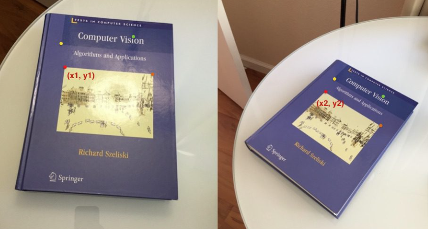
A homography transforms a square to arbitrary quad.

• Images of two planes are already related by a Homography
• We need 4 corresponding points to estimate Homography

Setup

---

import os
import cv2
import numpy as np
import matplotlib.pyplot as plt
import glob

from zipfile import ZipFile
from urllib.request import urlretrieve

%matplotlib inline

.

Download Assets

def download_and_unzip(url, save_path):
    print(f"Downloading and extracting assests....", end="")

    # Downloading zip file using urllib package.
    urlretrieve(url, save_path)

    try:
        # Extracting zip file using the zipfile package.
        with ZipFile(save_path) as z:
            # Extract ZIP file contents in the same directory.
            z.extractall(os.path.split(save_path)[0])

        print("Done")

    except Exception as e:
        print("\nInvalid file.", e)

URL = r"https://www.dropbox.com/s/zuwnn6rqe0f4zgh/opencv_bootcamp_assets_NB8.zip?dl=1"

asset_zip_path = os.path.join(os.getcwd(), "opencv_bootcamp_assets_NB8.zip")

# Download if assest ZIP does not exists. 
if not os.path.exists(asset_zip_path):
    download_and_unzip(URL, asset_zip_path)   

Read Image

---

# Read reference image
#Remember that opencv uses BGR instead of RGB so if we plot the image before converting over to RGB you'll see what it looks like below
refFilename = "form.jpg"
print("Reading reference image:", refFilename)
im_1 = cv2.imread(refFilename, cv2.IMREAD_COLOR)
im1 = cv2.cvtColor(im_1, cv2.COLOR_BGR2RGB)

# Read image to be aligned
imFilename = "scanned-form.jpg"
print("Reading image to align:", imFilename)
im2 = cv2.imread(imFilename, cv2.IMREAD_COLOR)
im2 = cv2.cvtColor(im2, cv2.COLOR_BGR2RGB)

# Display both images, note the subplot() has arguments of: rows, columns, index number
plt.figure(figsize=[20, 10]); 
plt.subplot(131); plt.axis('off'); plt.imshow(im_1); plt.title("Before Conversion")
plt.subplot(132); plt.axis('off'); plt.imshow(im1); plt.title("Original Form")
plt.subplot(133); plt.axis('off'); plt.imshow(im2); plt.title("Scanned Form")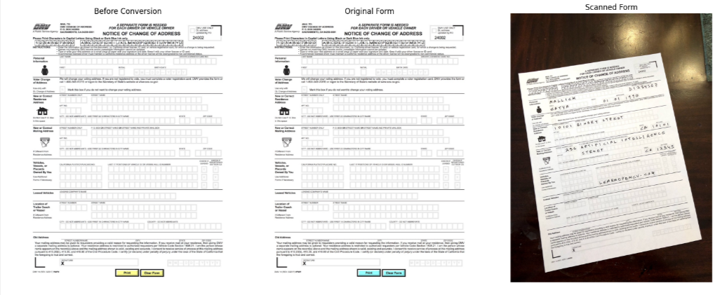

Find Keypoints

---

Note that the more keypoints we can find the more accurate our transformation will be.

1. First we will convert both images to grayscale because the code requires grayscale images
2. Create an orb class, which is extracting features from images, features that relate to that specific image itself
3. Use the orb object to detect keypoints and descripters for each image
4. Keypoints are associated with sharp edges and shapes and there is a list of descriptors associated with each keypoint which is a vector which describes the region around that keypoint
5. So we can use the descriptors of two edges to compare them
6. Keypoints are the red circle, along with their centers and the descriptors describe the patch where that keypoint is located
7. List of keypoints for fig 1 & 2 are overlapping, and so we will try to find the one in common that match so we can align the new image

# Convert images to grayscale
im1_gray = cv2.cvtColor(im1, cv2.COLOR_BGR2GRAY)
im2_gray = cv2.cvtColor(im2, cv2.COLOR_BGR2GRAY)


# Detect ORB features and compute descriptors.
MAX_NUM_FEATURES = 500
orb = cv2.ORB_create(MAX_NUM_FEATURES)
keypoints1, descriptors1 = orb.detectAndCompute(im1_gray, None)
keypoints2, descriptors2 = orb.detectAndCompute(im2_gray, None)

# Display
im1_display = cv2.drawKeypoints(im1, keypoints1, outImage=np.array([]), 
                                color=(255, 0, 0), flags=cv2.DRAW_MATCHES_FLAGS_DRAW_RICH_KEYPOINTS)

im2_display = cv2.drawKeypoints(im2, keypoints2, outImage=np.array([]), 
                                color=(255, 0, 0), flags=cv2.DRAW_MATCHES_FLAGS_DRAW_RICH_KEYPOINTS)

plt.figure(figsize=[20,10])
plt.subplot(121); plt.axis('off'); plt.imshow(im1_display); plt.title("Original Form");
plt.subplot(122); plt.axis('off'); plt.imshow(im2_display); plt.title("Scanned Form");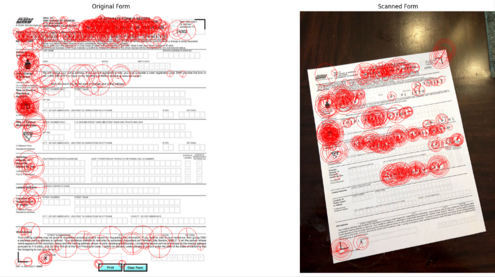

Match Keypoints

---

# Match features.
matcher = cv2.DescriptorMatcher_create(cv2.DESCRIPTOR_MATCHER_BRUTEFORCE_HAMMING)

# Converting to list for sorting as tuples are immutable objects.
matches = list(matcher.match(descriptors1, descriptors2, None))

# Sort matches by score
matches.sort(key=lambda x: x.distance, reverse=False)

# Remove not so good matches to only the top 10%
numGoodMatches = int(len(matches) * 0.1)
matches = matches[:numGoodMatches]

# Draw top matches between the two images. If the descriptors match close enough a keypoint match is drawn. There are some false positive but we still have a large number of true matches to accomplish the conversion
im_matches = cv2.drawMatches(im1, keypoints1, im2, keypoints2, matches, None)

plt.figure(figsize=[40, 10])
plt.imshow(im_matches);plt.axis("off");plt.title("Original Form")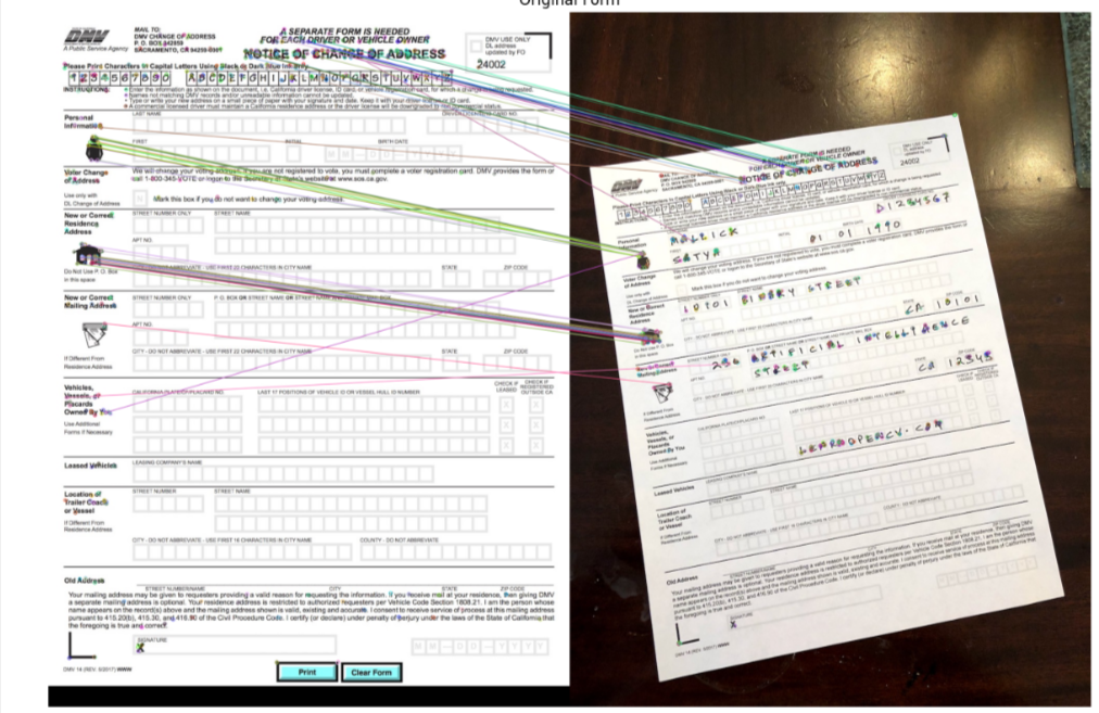

Find Homography

---

# Extract location of good matches
points1 = np.zeros((len(matches), 2), dtype=np.float32)
points2 = np.zeros((len(matches), 2), dtype=np.float32)

for i, match in enumerate(matches):
    points1[i, :] = keypoints1[match.queryIdx].pt
    points2[i, :] = keypoints2[match.trainIdx].pt

# Find homography using the RANSAC algorithm
h, mask = cv2.findHomography(points2, points1, cv2.RANSAC)

Warp Image

---

# Pass the homography to warp image
height, width, channels = im1.shape
im2_reg = cv2.warpPerspective(im2, h, (width, height))

# Display results
plt.figure(figsize=[20, 10])
plt.subplot(121);plt.imshow(im1);    plt.axis("off");plt.title("Original Form")
plt.subplot(122);plt.imshow(im2_reg);plt.axis("off");plt.title("Scanned Form")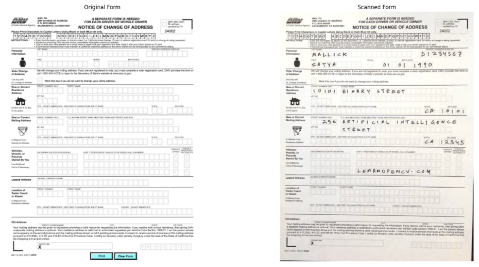

So as you can see we’ve changed the outlook of the uploaded image, and now we can process the form automatically

Panorama

---

It is advisable to use the same light setting, and a fixed camera position to take the multitude of images to stitch to form a panorama view. This is similar to image alignment above except that we will use the stitching function once we find the keypoints.’

Import Assets

URL = r"https://www.dropbox.com/s/0o5yqql1ynx31bi/opencv_bootcamp_assets_NB9.zip?dl=1"

asset_zip_path = os.path.join(os.getcwd(), "opencv_bootcamp_assets_NB9.zip")

# Download if assest ZIP does not exists.
if not os.path.exists(asset_zip_path):
    download_and_unzip(URL, asset_zip_path)

Here are the steps needed to create a panorama view:

1. Find keypoints in all images
2. Find pairwise correspondences
3. Estimate pairwise Homographies
4. Refine Homographies
5. Stitch with Blending

# Read Images

imagefiles = glob.glob(f"boat{os.sep}*")
imagefiles.sort()


images = []
for filename in imagefiles:
    img = cv2.imread(filename)
    img = cv2.cvtColor(img, cv2.COLOR_BGR2RGB)
    images.append(img)

num_images = len(images)

import math

# Display Images
plt.figure(figsize=[30, 10])
num_cols = 3
num_rows = math.ceil(num_images / num_cols)
for i in range(0, num_images):
    plt.subplot(num_rows, num_cols, i + 1)
    plt.axis("off")
    plt.imshow(images[i])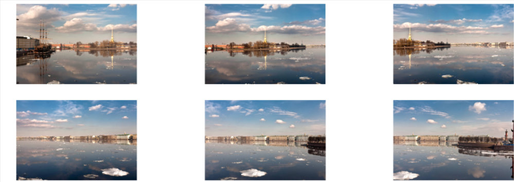

# Stitch Images using sticher class
stitcher = cv2.Stitcher_create()
status, result = stitcher.stitch(images)

if status == 0:
    plt.figure(figsize=[30, 10])
    plt.imshow(result)