~AI\computer_vision\od_projects\opencv_learn>venv_opencv\Scripts\activate

(venv_opencv) ~AI\computer_vision\od_projects\opencv_learn>jupyter notebookImage Manipulation
In this page we will cover how to perform image transformations including:
- Accessing and manipulating images pixels
- Image resizing
- Cropping
- Flipping
Setup
Reminder:
- Since I am trying to keep all notebooks organized I will go into my directory
- Activate the appropriate venv_opencv
- From an activated venv I will open jupyter notebook (see the code below)
- Create a new notebook: image_manipulation_opencv
- Choose “Py venv_opencv” kernel
.
Import Libraries
import os
import cv2
import numpy as np
import matplotlib
import matplotlib.pyplot as plt

from zipfile import ZipFile
from urllib.request import urlretrieve

from IPython.display import Image

%matplotlib inline
Import Assets
def download_and_unzip(url, save_path):
    print(f"Downloading and extracting assests....", end="")

    # Downloading zip file using urllib package.
    urlretrieve(url, save_path)

    try:
        # Extracting zip file using the zipfile package.
        with ZipFile(save_path) as z:
            # Extract ZIP file contents in the same directory.
            z.extractall(os.path.split(save_path)[0])

        print("Done")

    except Exception as e:
        print("\nInvalid file.", e)
# provide url and call function
URL = r"https://www.dropbox.com/s/rys6f1vprily2bg/opencv_bootcamp_assets_NB2.zip?dl=1"
asset_zip_path = os.path.join(os.getcwd(), "opencv_bootcamp_assets_NB2.zip")
# Download if assest ZIP does not exists.
if not os.path.exists(asset_zip_path):
download_and_unzip(URL, asset_zip_path) Access Pixels
We’ll look at the same image we use in the previous section, if you recall
- We’ll read it using Opencv
- Plot it with matplotlib showing the pixels
- Print the image for clarification
- As you can see it is clear how to access each pixel, remember it is zero based indexing
# Read image as gray scale.
cb_img = cv2.imread("checkerboard_18x18.png", 0)

# Set color map to gray scale for proper rendering.
plt.imshow(cb_img, cmap="gray")
print(cb_img)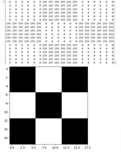
- For accessing any pixel in a numpy matrix, you have to use matrix notation such as matrix[r,c], where the r is the row number and c is the column number. Also note that the matrix is 0-indexed.
- For example, if you want to access the first pixel, you need to specify matrix[0,0]. Let us see with some examples. We will print one black pixel from top-left and one white pixel from top-center.
- As you can see the first cell is 0 which is black, second value is for the upper left corner of the white box. So it’s the first row of the 7 column
# print the first pixel of the first black box, First C in First R (upper left corner)
print(cb_img[0, 0])
# print the first white pixel to the right of the first black box
print(cb_img[0, 6])

# OUTPUT
0
255
Modify Pixels
- It is always best to make a copy of the image before modifying it
cb_img_copy = cb_img.copy()
cb_img_copy[2, 2] = 200
cb_img_copy[2, 3] = 200
cb_img_copy[3, 2] = 200
cb_img_copy[3, 3] = 200

# Same as above using slicing instead of explicit assignments
# cb_img_copy[2:3,2:3] = 200

plt.imshow(cb_img_copy, cmap="gray")
print(cb_img_copy)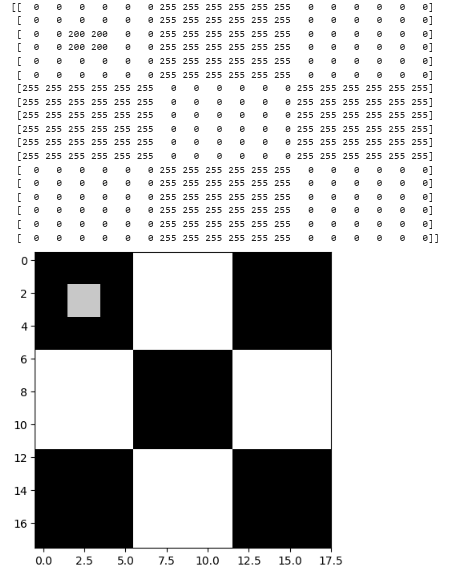
Cropping Images
Cropping an image is simply achieved by selecting a specific (pixel) region of the image.
- Read in a colored image
- SWAP channels to RGB
- Display using matplolib
img_NZ_bgr = cv2.imread("New_Zealand_Boat.jpg", cv2.IMREAD_COLOR)
img_NZ_rgb = img_NZ_bgr[:, :, ::-1]

plt.imshow(img_NZ_rgb)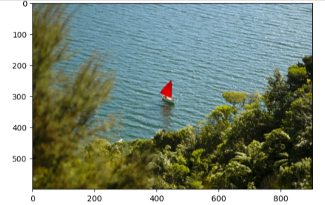
- In order to crop we use slicing as we would any array
- Assign to a copy not to itself to maintain the original
- If we want to start at row 200 to row 400
- Column 300 to 600
Remember Rows start from UPPER LEFT at zero, Columns start from LOWER LEFT
cropped_region = img_NZ_rgb[200:400, 300:600]
plt.imshow(cropped_region)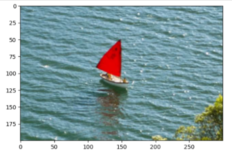
Resize
The function resize resizes the image src down to or up to the specified size. The size and type are derived from the src,dsize,fx, and fy. resize(): Documentation link
Function Syntax
dst = resize( src, dsize[, dst[, fx[, fy[, interpolation]]]] )dst: output image; it has the size dsize (when it is non-zero) or the size computed from src.size(), fx, and fy; the type of dst is the same as of src.
The function has 2 required arguments:
src: input imagedsize: output image size
Optional arguments that are often used include:
fx: Scale factor along the horizontal axis; when it equals 0, it is computed as (𝚍𝚘𝚞𝚋𝚕𝚎)𝚍𝚜𝚒𝚣𝚎.𝚠𝚒𝚍𝚝𝚑/𝚜𝚛𝚌.𝚌𝚘𝚕𝚜fy: Scale factor along the vertical axis; when it equals 0, it is computed as (𝚍𝚘𝚞𝚋𝚕𝚎)𝚍𝚜𝚒𝚣𝚎.𝚑𝚎𝚒𝚐𝚑𝚝/𝚜𝚛𝚌.𝚛𝚘𝚠𝚜
The output image has the size dsize (when it is non-zero) or the size computed from src.size(), fx, and fy; the type of dst is the same as of src.
Specify Scaling Factor fx & fy
- We will use the same cropped image from above and since we are using a factor of 2 in both directions, of course the image will be twice as wide and twice as tall. You can see from the dimensions below
resized_cropped_region_2x = cv2.resize(cropped_region, None, fx=2, fy=2)
plt.imshow(resized_cropped_region_2x)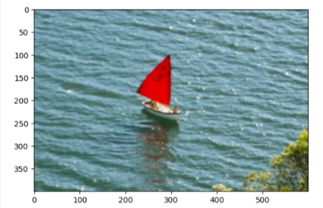
Specify Exact Size
- As you would guess, we have to be careful here that we don’t mess the aspect ratio, unless we are intentionally trying to exactly that
desired_width = 100
desired_height = 200
dim = (desired_width, desired_height)

# Resize background image to sae size as logo image
resized_cropped_region = cv2.resize(cropped_region, dsize=dim, interpolation=cv2.INTER_AREA)
plt.imshow(resized_cropped_region)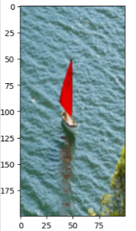
Maintain Aspect Ratio
- We can use dsize to work with the aspect ratio
- Here we want to keep the width at 100 but want to maintain the aspect ratio, so we can calculate the aspect ratio based on the fixed desired width
- We can access the image width from the shape[1] and image height from shape[0]
- So as you see in the image below the height turns out to be about 67px while the width is set at 100px
desired_width = 100
aspect_ratio = desired_width / cropped_region.shape[1]
desired_height = int(cropped_region.shape[0] * aspect_ratio)
dim = (desired_width, desired_height)

# Resize image
resized_cropped_region = cv2.resize(cropped_region, dsize=dim, interpolation=cv2.INTER_AREA)
plt.imshow(resized_cropped_region)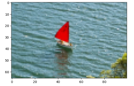
Save & Display
Cropped & Resized
- Remember we have to swap channels
- Let’s see if we don’t swap channels
# Save resized image to disk
cv2.imwrite("resized_cropped_region_2x.png", resized_cropped_region)

# Display the cropped and resized image
Image(filename="resized_cropped_region_2x.png")
What happened?
- Remember that OpenCv works with BGR and NOT RGB
- So we have to reverse the order
- Write it to disk an save it as filename
- Display the image
# Swap channel order
resized_cropped_region_2x = resized_cropped_region_2x[:, :, ::-1]

# Save resized image to disk
cv2.imwrite("resized_cropped_region_2x.png", resized_cropped_region_2x)

# Display the cropped and resized image
Image(filename="resized_cropped_region_2x.png")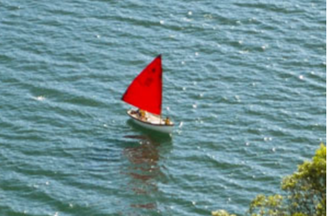
Cropped
The image above is the cropped and resized image, let’s do the same on the cropped image that wasn’t resized, which should give us the smaller size
# Swap channel order
cropped_region = cropped_region[:, :, ::-1]

# Save cropped 'region'
cv2.imwrite("cropped_region.png", cropped_region)

# Display the cropped and resized image
Image(filename="cropped_region.png")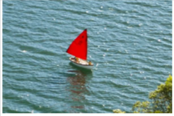
Flipping Images
- This is pretty straight forward again by using the function: flip()
dst = cv.flip( src, flipCode )dst: output array of the same size and type as src.
The function has 2 required arguments:
src: input imageflipCode: a flag to specify how to flip the array; 0 means flipping around the x-axis and positive value (for example, 1) means flipping around y-axis. Negative value (for example, -1) means flipping around both axes.
img_NZ_rgb_flipped_horz = cv2.flip(img_NZ_rgb, 1)
img_NZ_rgb_flipped_vert = cv2.flip(img_NZ_rgb, 0)
img_NZ_rgb_flipped_both = cv2.flip(img_NZ_rgb, -1)

# Show the images
plt.figure(figsize=(18, 5))
plt.subplot(141);plt.imshow(img_NZ_rgb_flipped_horz);plt.title("Horizontal Flip");
plt.subplot(142);plt.imshow(img_NZ_rgb_flipped_vert);plt.title("Vertical Flip");
plt.subplot(143);plt.imshow(img_NZ_rgb_flipped_both);plt.title("Both Flipped");
plt.subplot(144);plt.imshow(img_NZ_rgb);plt.title("Original");