~\AI\computer_vision>python
Python 3.11.8 (tags/v3.11.8:db85d51, Feb  6 2022, 22:03:32) [MSC v.1937 64 bit (AMD64)] on win32
Type "help", "copyright", "credits" or "license" for more information.
>>>exit()Computer Vision Overview
Object Detection
In the world of machine learning and computer vision, the process of making sense out of visual data is called ‘inference’ or ‘prediction’. I’ll cover a few models, one of which is YOLO (you only look once) which offers different versions tailored for high-performance, real-time inference on a wide range of data sources.
Such models are capable of predicting for various inference needs:
- Versatility - capable of making inferences on images, videos, and live streams
- Performance - engineered for real-time, high speed processing without sacrificing accuracy
- Ease of use - intuitive Python and CLI interfaces for rapid deployment and testing
- Highly Customizable - various settings and parameters to tune the models’ inference behavior
In order to learn about Object Detection OD we will learn about localization first:
Classification
This is when a network looks at an image and classifies it as a car, or cat or….. but in order to understand OD we need to learn about localization
Localization
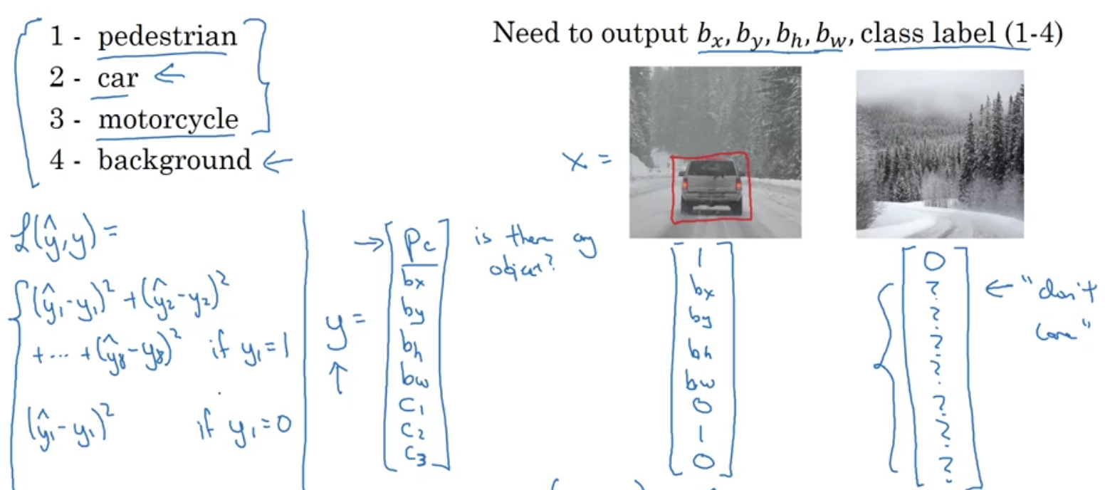
We not only have to classify an object as what it is but it also has to put a bounding box around the image that it classified. In other words, where in the image is the object located.
The network can detect several objects but each object has to have its own localization (location on the image)
- The way we achieve this is by outputing the location as well as the classification (probability of a class label = Pc)
- Now our output will contain bx, by, bh, bw
- We also need to output the class is belongs to as in C1…Cx x being the number of classes available
- Here below if an object is detected Pc= 1 and if not object exists then Pc=0 and we don’t care what the other parameters are since no object is detected
- The Loss Function if an object is detected would be the difference between the Detected Object and the True Object
Landmark Detection
Let’s say we are building a face part recognition, and we want to know the location of each corner of the eyes, this is called landmark location detection.
We can start by selecting a number of landmarks and generate a label training sets that contains all these landmarkds. Then we can have a NN tell us where all the landmarks are on the face.
Sliding Window
Let’s say we want to create an OD NN, we can start with
- A training set x: closely cropped images of cars
- y: a binary 1 or 0 value if it is a car or not
- Then we can just input an image and the ConvNet will output a 0 or 1 for a car or not
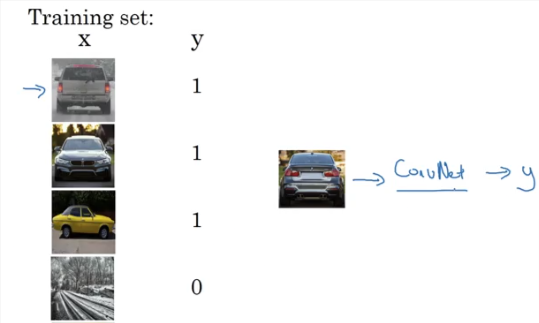
- Then you can choose a window size feed it through a ConvNet and have it slide over the image and then increase the size of the window and run it again and again and have it predict a value of 0 or 1 for each cell
- The disadvantages of such a model is computation costs
We can implement a sliding window into a Conv layer here is an image of how a FC network can be transformed to convolutional layers
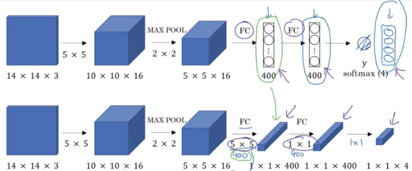
So how do we convert our sliding window network into a Convolution implementation, if we have a 16x16x3 image and we run our 14x14x3 window over it which will need to run 4 times. We realize that most of the cells are duplicated. So we share outputs and we can run the entire picture by combining all the windows together in one pass and process the result
R-CNN Region Proposal
Some parts of the input image will be blank or not have any objects in it, so instead of running our sliding window algorithm over the entire image we can specify which region we want to run the sliding window algo.
The way it works is by running a segmentation algorithm which finds a blob in the image and directs the sliding window to run there.

- So you run the segmentation algorithm and find the blobs as shown below then run the sliding window to detect objects in those regions
- So possibly you find 2000 blobs then you can focus on those blobs
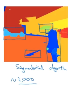
- R-CNN is pretty slow because it classify proposed regions one at a time. Output label & bounding box
- Fast R-CNN uses conv implementation of sliding windows to classify all the proposed regions
- Faster R-CNN uses conv network to propose regions
All of the R-CNN are still slower than the YOLO covered below and ahead in other sections
Semantic Segmentation U-Net
This is a more sophisticated algorithm that draws an outline around an object instead of a bounding box. This is based on pixel by pixel this way you know exactly which pixel belongs to the object.
- This is a very useful algorithm in commercial use because if you are running a self-driven car we don’t want to detect a road
- We want to detect the exact pixels that are safe to drive over.
- Medical imaging is a major use of this as well, if we wanted to spot irregularities in imagings, X-Rays and so forth, this algorithm will color the region a certain color so we can distinguish the difference and catch diseases
- In the image below, we can have the algorithm detect the tumor and color it in a way that separates each pixel from the rest of the image

- Let’s say we want to segment out the car from this image, so the algorithm will output a 1 for each pixel in the car and 0 for other
- Can do the same for building, road…..
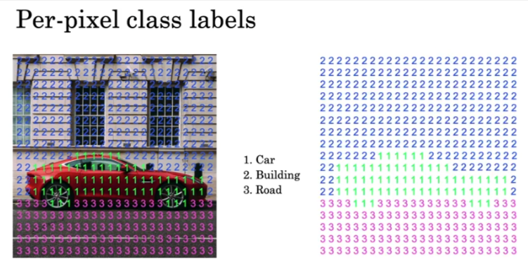
- U-net will generate a whole matrix of class labels
- We input the image, and we change the last 3 layers to instead of reducing the output we want to expand it back up so we can pick up the minor details of each pixel
- So as we go deeper into the U-Net network the output unit will go back up

- While the number of channels will decrease until the output is the same size as the input and we end up with a segmentation of the input

- So what does it take to make the output increase in size in the last layers?
- We have to use Transpose Convolutions
Transpose Convolutions U-Net
So as we covered above, in order to expand the output of a Conv Network back to the initial size of the input we have to use Transpose Convolution

- Above is a recap of Normal Convolution as we covered before
- In a Transpose Conv, we might input a 2x2 set of activations -> 3x3 filter -> 4x4 that’s bigger than the original input
- So here is how it is done:
- 2x2 input
- 3x3 filter
- padding =1 (is applied to the output not input as we did in normal ConvNet)
- stride =2
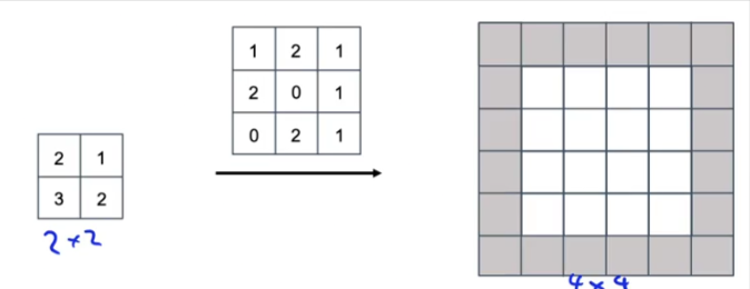
- If you remember in Normal Conv we overlay the filter over the input and use stride to move it around
- In Transpose Conv we overlay the filter on the empty OUTPUT and make our calculations
- Here is how it’s done
- We take the first upper left cell 2
- Multiply it by every cell in the filter
- Save the results in the 3x3 transposed filter that’s overlaid over the output starting in the upper left corner
- The padding area WILL NOT contain any values, so we just use the results from the lower right 4 cells from the filter and place them in the corresponding cells in the output
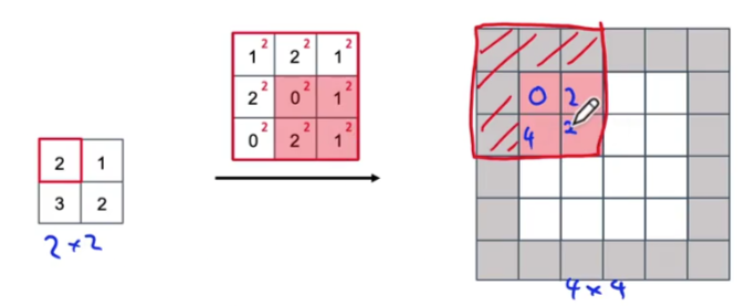
- Now you carry this process colored in green
- Since we are using a stride=2 then our output box will move to the right by 2 cells
- Again, the padding will not take any values
- Note that the two lower rows from the filter will overlap previous values calculated from above
- In that case we simply add the green value to the red value from above and enter the results in the grid
- Now as you can see below that we have exhausted the row 1 values from the input and we have also filled all the output values in the first 2 rows of the output (padding surrounding them is not to be filled)
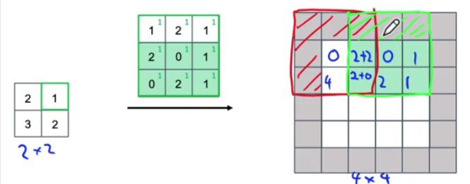
- Remember we have stride= 2 so when we calculate the lower row in the input we have to move the output transposed 3x3 by 2 cells down
- We repeat the steps from above and we end up with
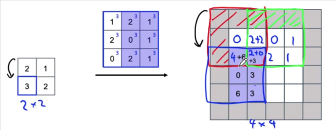
- One last time and we end up with
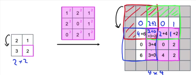
U-Net
Is one of the important algorithms used today as it narrows the object detected to pixels

Let’s lay out the U-Net architecture that’s responsible for Semantic Segmentation and Transpose Convolutions
- The first 3 layers use Normal Conv and the latter part of the NN uses Transpose Conv
- But what if we can skip from the first layer to the fifth layer where the sizes are the same? Is that more efficient?
- There is a skip connection which accomplish that, it passes the overall generalized features of what it detected as being a cat and it passes it directly to the fifth layer (which is the same size)
- The fifth layer can now have access to the overall generailzed features of what’s a cat in the image from layer 1, as well as the finite details from layer 4 and combines the two for more accurate outpu

Architecture
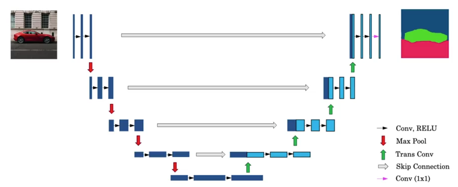
- Above is the overall architecture of U-Net, Let’s go through the general details
- This was generally created for biomedical image segmentation or semantic segmentation overall
- Input is HxWx3 so let’s just look at it from the profile of the channel side that’s why it appears as a rectangle
- Is fed to 3 Conv Relu layers
- Then we use MaxPool to reduce the size and then feed it through 3 Relu Layers
- Then apply MaxPool again to reduce it, and again to reduce it to the lowest set of the layers
- At the bottom we feed it through 2 more Relu ConvNet layers and we end up at the bottom right of the image above
- So far it is a Normal ConvNet with a very small outputs at the bottom
- At the bottom right we feed it through the first Transpose Conv layer, we did not increase the size we just added more channels and as you see the size is still the same as below.
- What you also do is apply the skip method which will take the set of features on the far right of the left side of the U and copy it over to the leftmost side of the right leg of the U
- So as you see there, you have a dark blue and light blue set of features combined together. The light blue part comes over from the Transpose Conv from below and the dark blue part comes over from the left
- That’s fed through 2 Normal Conv Relu Layers
- Then we apply a Trans Conv to the output and is shown in the up arrow in the image
- Here again a skip method is added which copies over the far right Normal Conv features from the left leg of the U
- Now the size is increased , on and on till we end up with the output
- Finally at the end we use a 1x1 Conv as shown in the magenta arrow to give us the output with the same dimensions as the input and the third dimension will be equal to the number of classes in the image.
- So if we are trying to find these classes: car, building, road then the size will be HxWx3 and we have 19 classes to search for then the output size will be HxWx19
YOLO
Bounding Box
Sliding window computation does not output an efficient process compared to a bounding box. A good way to have an efficient bounding box we can use YOLO algorithm.
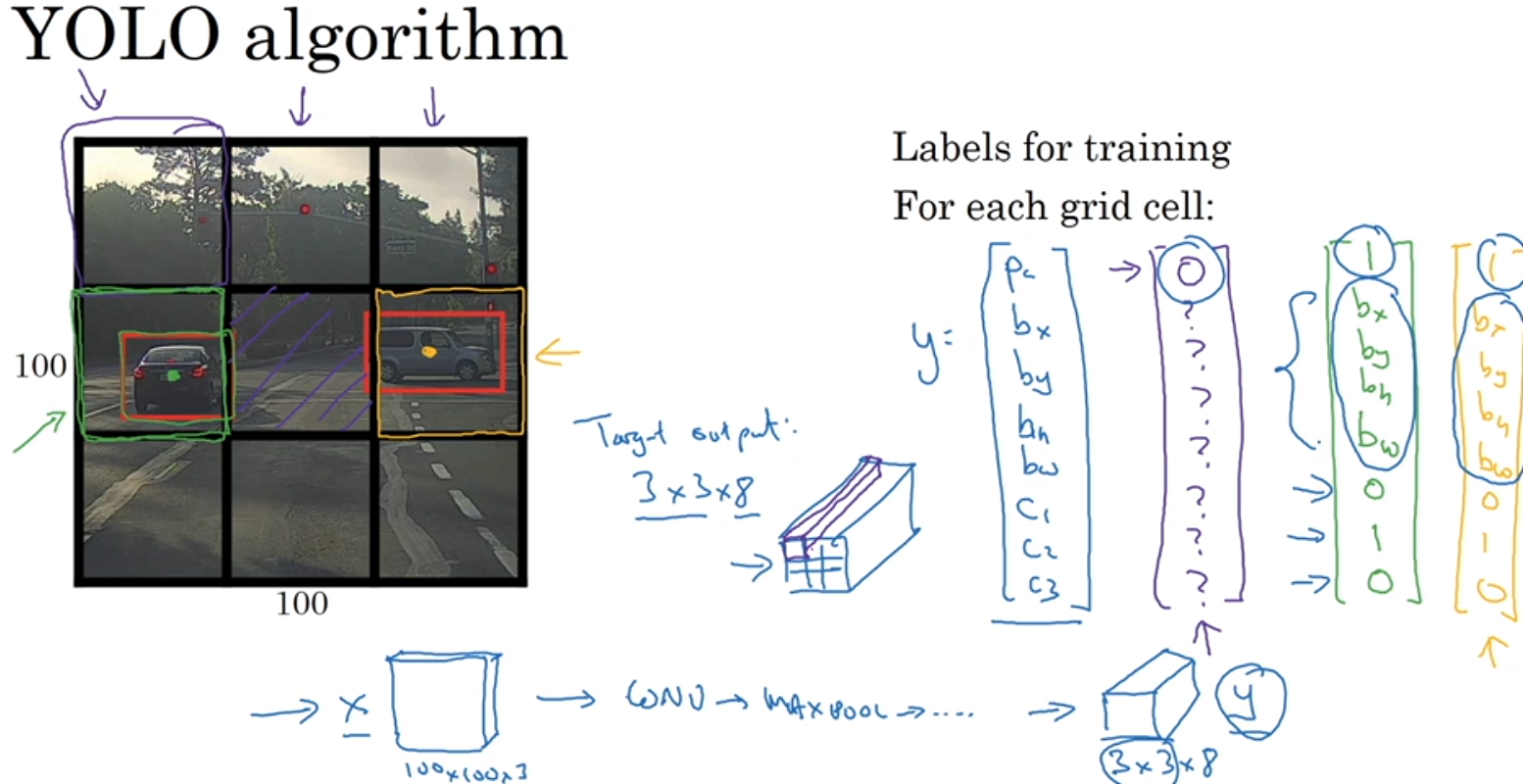
- You divide the image into a grid cell
- For each of the 9 cells you assign a label y which contains the output of Pc, bx, by, bh, bw, C…
- Cs stand for classes of : pedestrian, motorcycle, car
- Yolo takes the midpoint of the bounding box and assigns it to the grid cell it is in
- It can only be assigned to one grid cell
- Sometimes a grid cell will have part of a detected object but if it doesn’t contain the midpoint it will shown as not containing a detected object
- So each grid cell will have an 8 dimensional output vector
- If the image contains 9 grid cells, then the Total output target will have a dimension of 3x3x8 output vector
- So now our input is 100x100x3 fed into ConvNet fed into Max Pool -> output a 3x3x8 volume vector y
- You can also use a much finer grid such as a 19x19 to eliminate or decreases, two objects midpoints appearing in the same grid cell
- You are not running the algorithm over and over again 9 times for 9 grid cells, we are only running it once
Encoding BBoxes
- Since some of the boxes extend into other cells we specify a factor or fraction of the overall width of the grid cell
- This way it can extend into other cells even if the midpoint is in another cell
- A fraction could be such as 0.9 or 0.3 or whatever of a grid cell width or height
Evaluation
How do you tell if the OD algorithm is accurate? To evaluate the accuracy of the od model we have to look at two items:
- How good is the location: IoU is used
- How good is the classification: mAP is used
IoU
IoU is used to measure the localization. Intersection over Union. It tells us how close the predicted bounding box is to the actual one
- It is measure by a value between 0-1. If IoU = 1 it means the two boxes are exactly the same
- If the two boxes overlap it will tells how much overlap is
- Correct if IoU >= 0.5 or it’s up to your application
IoU is the overlap between two bounding boxes
IoU = Area of Intersection/Area of Union
Average Precision
To understand precision we have to understand confusion matrix, precision, and recall
Confusion Matrix
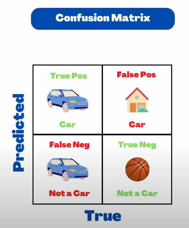
Is simply a table displaying one one side the the predicted values compared to the actual values. The table above shows starting in the upper left corner,
- Upper left: The actual class is Car and the predicted value is car -> True Positive (correct prediction of positively identification)
- Upper right: Actual class is house, predicted value is car -> False Positive (wrong prediction of positive)
- Lower left: Actual class is car, predicted not a car -> False Negative (wrong prediction of negation)
- Lower right: Actual class is ball, predicted not a car -> True Negative (which is tjhe correct prediction of negation), this value is not used in the calculations and is usually attributed to noise
Precision
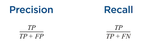
Precision = Actual Positive Detections out of the total Positive Predictions = True Positives/(True Positives+False Positives)
Recall
Recall = Actual Positive Detections out of all Predictions = True Positives/(True Positives+False Negatives)
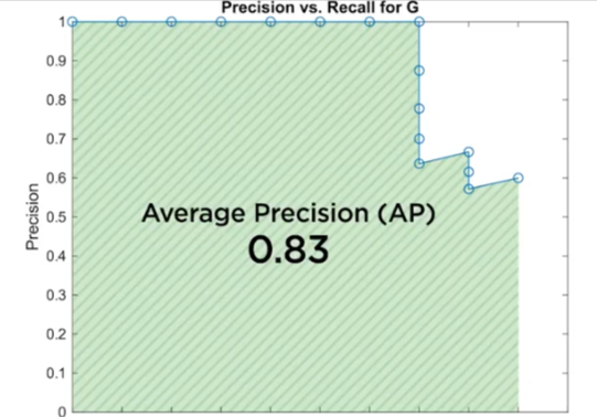
Combining the two above gives us the Average Precision which is the area under the Precision VS Recall curve
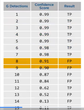
- Or you can look at a table run at a low confidence level say 0.05 then for each class sort by decreasing scores.
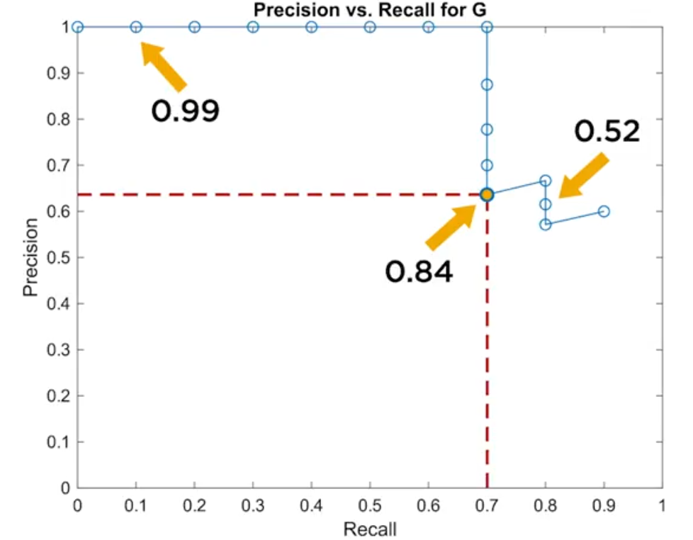
- Then plot a P vs R graph.
- The curve always starts at 0,1 as is the first line which is the result of the first top 10 TP results (the first 9 are shown in the table below out of 10)
- The second detection is a TP as well and will be plotted next to it to the right and on and on till we get to the first FP which is detection 8 which would be the ninth point on the plot
- Since we have detected 7 out of 10 so far then Recall = 0.7
- Next prediction is FP so we drop one level on the precision axis but recall is still 0.7 till we get to
- The next TP detection 12 and we move the line to the right to show recall=0.8 an increase and we also increase Precision and so on till the curve is complete
- So at the end you know it will impossible to get a precision of 1 so we could set our goals at a recall=0.7
- The graph is just for the letter G
- We have to calculate one for each class in the dataset and then come up with the mean average precision for all combined
If we have multiple classes then we take the Mean Average Precision = mAP for all classes, which will give us the accuracy of the model. The curve maximizes the effects of both matrices and gives us a better idea of the accuracy of the model
Average Precision
Now we can calculate the area under the curve and we get AP.
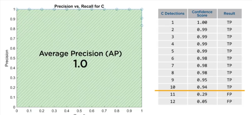
Here are some plots for some other classes. Note for class C it is possible to have a recall of 1 since we predicted the first 10 as TP, but precision drops after the 10th prediction, but that doesn’t affect the area under the curve
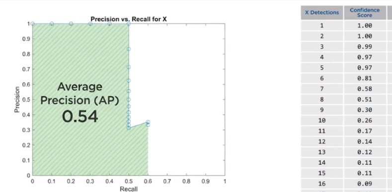
Here is the plot for class X where it detects the first 5 as TP and then it detects a whole string of FP to drive the precision down and we end up with an AP = 0.54
To evaluate the effectiveness of the model for all classes, you take the mean of all Average Precision mAP in the case above it comes out to 0.8
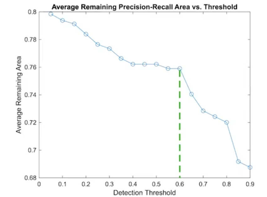
- It is best to run the detector for a range of threshold values and create new precision recall curves for each class.
- The area under the curves will decrease as the threshold increases.
- The goal is to see the relationship between the area decreases and threshold increases by averaging the area across all classes.
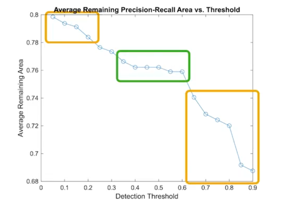
- So you choose a point close to this point will maximize the model efficiency
Non-Max Suppression
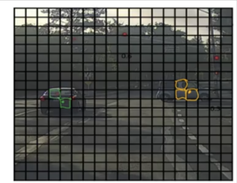
Often you’ll find that your algorithm may detect the same object more than once.
- If we setup a grid of size 19x19 many of the cells will detect an object in it with a mid point in each of the cells
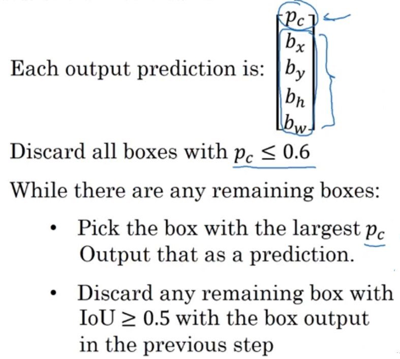
- Non-max suppression will clean up these detections based on the maximum probability of detections
- Once the max value detection is highlighted, then the remaining ones with a high IoU (which means they overlap the max bounding box alot) will be eliminated.
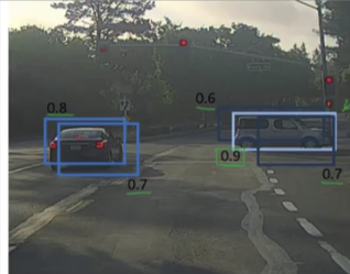
- So we eliminate the lower probability boxes and
- Supress the non-max probability boxes
Anchor Box
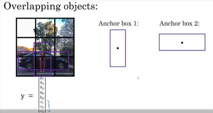
We covered anchor boxes in CNN here we will incorporate them into the algorithm
- Anchor box: each object in training image is assigned to grid cell that contains that object’s midpoint
- We create a y label for each anchor box so here we will have Y1 and Y2 both inside Y as shown below so Y has 16 values
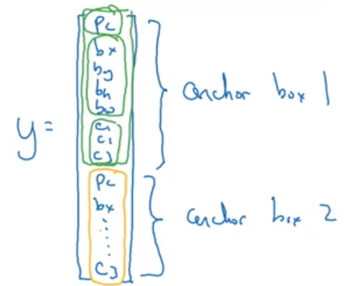
- With two anchor boxes: each object in training image is assigned to grid cell that contains object’s midpoint and anchor box for the grid cell with highest IoU
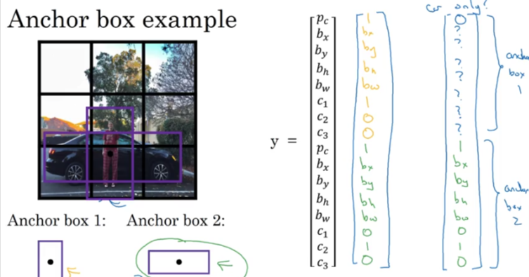
- Here below we assign pedestrian to the similar box which is box 1 and car to box 2
- If only a car is in the image, then the values for box 1 will have a value of 0 in Pc
Predictions
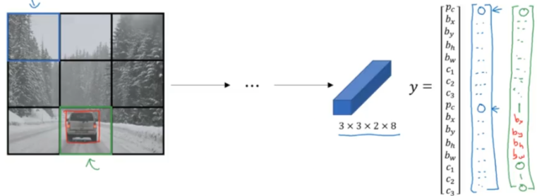
So the NN will make predictions based on the input image, in the example of the car above, it will output a 3x3x2x8 y which after being flattened out will tell us if an object was detected and the probability of that object being the class between 1 & 3
Basic Setup
Install Python
I’ll start with the basics.
- Install python
- Create a dedicated directory: ~/AI/computer_vision/od_projects/1_yolo_ocv_py
- Since we are going to be working with yolo, OpenCV and Python
- I will use a combination of three: jupyter notebook, quarto & pycharm
- Since I already have python installed let’s verify the version
.
Setup Virtual Environment
- Let’s go into the directory and create a virtual environment
- Go into the directory/folder, type cmd >
- Use python -m venv …. to create a new virtual environment named: venv_1_yolo_ocv_py which stands for virtual env #1 using yolo, Opencv and Python
- After a few seconds we will be returned to the prompt and if you check your folder you’ll find the new environment was created
# From within quarto I can use
py -m venv ~name of environment~

# Like this
~AI\computer_vision\od_projects\1_yolo_ocv_py> python -m venv venv1_yolo
Activate venv
- Now before we start any work we need to make sure we activate our venv and that way we can ensure all our work will be replicated
- Activate venv by going to the directory/folder where it is located, call it by name along with the following
~\Scripts\activate - It will respond with a prompt listing the name of the venv first before the prompt
~\AI\computer_vision\od_projects\1_yolo_ocv_py>venv1_yolo\Scripts\activate

(venv1_yolo) D:\AI\computer_vision\od_projects\1_yolo_ocv_py>
# If using Linux
source name_env/bin/activate
# Using windows cmd
name_env\Scripts\activate.bat
# Using windows powershell
name_env\Scripts\activate.ps1Create Requirements Folder
- In the same folder where the venv is located let’s create a document to track all the requirements
- You can either do it in advance like the step above, but in most cases you might end up adding another requirement, so what I end up doing is installing what I think I need and if I ever install something else I will repeat this step
- Use this command to create the requirements text file, I attach the venv name to the file
# Linux
python3 -m pip freeze > venv_requirements.txt
# Windows
py -m pip freeze > venv_requrirements.txt
Install Requirements
- Make sure all the requirements are installed in the new venv
- If we created the list of requirements in the text file above and we want to install it
- Use the code below
- venv name is venv1_yolo
- requirements file is venv1_yolo_requirements.txt
(venv1_yolo) ~\AI\computer_vision\od_projects\1_yolo_ocv_py>pip install -r venv1_yolo_requirements.txt


Installing collected packages: pytz, PyQt5-Qt5, tzdata, six, PyQt5-sip, pyparsing, pillow, packaging, numpy, lxml, kiwisolver, fonttools, cycler, python-dateutil, pyqt5, opencv-python, contourpy, pandas, matplotlib, labelImg
Successfully installed PyQt5-Qt5 PyQt5-sip contourpy cycler fonttools kiwisolver labelImg lxml matplotlib numpy opencv-python packaging pandas pillow pyparsing pyqt5 python-dateutil pytz six tzdata

[notice] A new release of pip is available: 24.0 -> 24.3.1
[notice] To update, run: python.exe -m pip install --upgrade pip
Deactivate venv
- When done or if you are moving to another project make sure you deactivate the venv first
(venv1_yolo) ~:\AI\computer_vision>deactivateRestoring Environments
- To reproduce the environment on another machine
- Create the new venv
- Activate the new venv
- Use pip install using the from venv_requirements.txt as seen above
- Same command as installing requirements above
# Linux
python3 -m pip install -r venv_requirements.txt
# Windows
py -m install -r venv_requirements.txt
Jupyter Notebook
If we want to use jupyter notebook it would be much simpler if we create a jupyter kernel for each venv we create so we can use choose it from a dropdown when we are working on that specific project in that certain venv.
- To use jupyter notebook inside venv use this command while the venv is activated
# First install ipykernel in the venv. I had alot of issues with jupyter not finding cv2 even though you can see it in the lib/packages folder. So I had to delete everything and make sure to run this command which will install the ipykernel in the venv. After that it had no problem finding all the installed packages
(venv_opencv) ~\AI\computer_vision\od_projects\opencv_learn> pip install ipykernel

# Register the venv Kernel
(venv_opencv) ~\AI\computer_vision\od_projects\opencv_learn>python -m ipykernel install --user --name=venv_opencv --display-name "Py venv_opencv"
Installed kernelspec venv_opencv in C:\Users\EMHRC\AppData\Roaming\jupyter\kernels\venv_opencv

# Open jupyter notebook from inside the venv
(venv_opencv) ~\AI\computer_vision\od_projects\opencv_learn>jupyter notebook
To uninstall the kernel
jupyter-kernel-spec uninstall venv_opencvOpen Jupyter Notebook
Open the notebook and start the work. The notebooks will be saved in the same folder as the venv_opencv
Datasets
Ultralytics
Ultralytics (maker of YOLO) supports and provides various datasets to facilitate computer vision tasks. Many other companies provide datasets but here is a summary of the list provided by Ultralytics for object detection:
Object Detection
Bounding box object detection is a computer vision technique that involves detecting and localizing objects in an image by drawing a bounding box around each object.
Argoverse: A dataset containing 3D tracking and motion forecasting data from urban environments with rich annotations.
COCO: Common Objects in Context (COCO) is a large-scale object detection, segmentation, and captioning dataset with 80 object categories.
LVIS: A large-scale object detection, segmentation, and captioning dataset with 1203 object categories.
COCO8: A smaller subset of the first 4 images from COCO train and COCO val, suitable for quick tests.
COCO128: A smaller subset of the first 128 images from COCO train and COCO val, suitable for tests.
Global Wheat 2020: A dataset containing images of wheat heads for the Global Wheat Challenge 2020.
Objects365: A high-quality, large-scale dataset for object detection with 365 object categories and over 600K annotated images.
OpenImagesV7: A comprehensive dataset by Google with 1.7M train images and 42k validation images.
SKU-110K: A dataset featuring dense object detection in retail environments with over 11K images and 1.7 million bounding boxes.
VisDrone: A dataset containing object detection and multi-object tracking data from drone-captured imagery with over 10K images and video sequences.
VOC: The Pascal Visual Object Classes (VOC) dataset for object detection and segmentation with 20 object classes and over 11K images.
xView: A dataset for object detection in overhead imagery with 60 object categories and over 1 million annotated objects.
RF100: A diverse object detection benchmark with 100 datasets spanning seven imagery domains for comprehensive model evaluation.
Brain-tumor: A dataset for detecting brain tumors includes MRI or CT scan images with details on tumor presence, location, and characteristics.
African-wildlife: A dataset featuring images of African wildlife, including buffalo, elephant, rhino, and zebras.
Signature: A dataset featuring images of various documents with annotated signatures, supporting document verification and fraud detection research.
Medical-pills: A dataset containing labeled images of medical-pills, designed to aid in tasks like pharmaceutical quality control, sorting, and ensuring compliance with industry standards.
Instance Segmentation
Instance segmentation is a computer vision technique that involves identifying and localizing objects in an image at the pixel level.
COCO: A large-scale dataset designed for object detection, segmentation, and captioning tasks with over 200K labeled images.
COCO8-seg: A smaller dataset for instance segmentation tasks, containing a subset of 8 COCO images with segmentation annotations.
COCO128-seg: A smaller dataset for instance segmentation tasks, containing a subset of 128 COCO images with segmentation annotations.
Crack-seg: Specifically crafted dataset for detecting cracks on roads and walls, applicable for both object detection and segmentation tasks.
Package-seg: Tailored dataset for identifying packages in warehouses or industrial settings, suitable for both object detection and segmentation applications.
Carparts-seg: Purpose-built dataset for identifying vehicle parts, catering to design, manufacturing, and research needs. It serves for both object detection and segmentation tasks.
Pose Estimation
Pose estimation is a technique used to determine the pose of the object relative to the camera or the world coordinate system.
COCO: A large-scale dataset with human pose annotations designed for pose estimation tasks.
COCO8-pose: A smaller dataset for pose estimation tasks, containing a subset of 8 COCO images with human pose annotations.
Tiger-pose: A compact dataset consisting of 263 images focused on tigers, annotated with 12 keypoints per tiger for pose estimation tasks.
Hand-Keypoints: A concise dataset featuring over 26,000 images centered on human hands, annotated with 21 keypoints per hand, designed for pose estimation tasks.
Dog-pose: A comprehensive dataset featuring approximately 6,000 images focused on dogs, annotated with 24 keypoints per dog, tailored for pose estimation tasks.
Classification
Image classification is a computer vision task that involves categorizing an image into one or more predefined classes or categories based on its visual content.
Caltech 101: A dataset containing images of 101 object categories for image classification tasks.
Caltech 256: An extended version of Caltech 101 with 256 object categories and more challenging images.
CIFAR-10: A dataset of 60K 32x32 color images in 10 classes, with 6K images per class.
CIFAR-100: An extended version of CIFAR-10 with 100 object categories and 600 images per class.
Fashion-MNIST: A dataset consisting of 70,000 grayscale images of 10 fashion categories for image classification tasks.
ImageNet: A large-scale dataset for object detection and image classification with over 14 million images and 20,000 categories.
ImageNet-10: A smaller subset of ImageNet with 10 categories for faster experimentation and testing.
Imagenette: A smaller subset of ImageNet that contains 10 easily distinguishable classes for quicker training and testing.
Imagewoof: A more challenging subset of ImageNet containing 10 dog breed categories for image classification tasks.
MNIST: A dataset of 70,000 grayscale images of handwritten digits for image classification tasks.
MNIST160: First 8 images of each MNIST category from the MNIST dataset. Dataset contains 160 images total.
Oriented Bounding Boxes (OBB)
Oriented Bounding Boxes (OBB) is a method in computer vision for detecting angled objects in images using rotated bounding boxes, often applied to aerial and satellite imagery.
Multi-Object Tracking
Multi-object tracking is a computer vision technique that involves detecting and tracking multiple objects over time in a video sequence.