# Create venv
~AI\computer_vision\od_projects\opencv_learn>py -m venv venv_opencv

# Activate venv
~AI\computer_vision\od_projects\opencv_learn>venv_opencv\Scripts\activate

# Install matplotlib
(venv_opencv) ~AI\computer_vision\od_projects\opencv_learn>pip install matplotlib

# Install OpenCV
(venv_opencv) ~AI\computer_vision\od_projects\opencv_learn>pip install opencv-python

# Verify installation
(venv_opencv) ~AI\computer_vision\od_projects\opencv_learn>python
Python 3.12.2 (tags/v3.12.2:6abddd9, Feb  6 2024, 21:26:36) [MSC v.1937 64 bit (AMD64)] on win32
Type "help", "copyright", "credits" or "license" for more information.
>>> import cv2 as cv
>>> cv.__version__
'4.10.0'
>>>Images - Start
One of the technologies OpenCv provides is an algorithm for face recognition rated in the top 10 globally. We’ll get into that later, but for now we’ll learn the basics of OpenCV the largest computer vision library. It has more functionality than the PIL library but is more difficult to use.
All this code can be found in jupyter notebook: getting_started_opencv.ipynb
Install OpenCV
Create venv
Install OpenCV
- Let’s first create a directory and name it: opencv_learn
- Create a venv: venv_opencv
- Activate the venv
- Install OpenCV
.
Create Jupyter Kernel
- To use jupyter notebook inside venv use this command while the venv is activated
# First install ipykernel in the venv. I had alot of issues with jupyter not finding cv2 even though you can see it in the lib/packages folder. So I had to delete everything and make sure to run this command which will install the ipykernel in the venv. After that it had no problem finding all the installed packages
(venv_opencv) ~\AI\computer_vision\od_projects\opencv_learn> pip install ipykernel

# Register the venv Kernel
(venv_opencv) ~\AI\computer_vision\od_projects\opencv_learn>python -m ipykernel install --user --name=venv_opencv --display-name "Py venv_opencv"
Installed kernelspec venv_opencv in C:\Users\EMHRC\AppData\Roaming\jupyter\kernels\venv_opencv

# Open jupyter notebook from inside the venv
(venv_opencv) ~\AI\computer_vision\od_projects\opencv_learn>jupyter notebook
To uninstall the kernel
jupyter-kernel-spec uninstall venv_opencvOpen Jupyter Notebook
Open the notebook and start the work. The notebooks will be saved in the same folder as the venv_opencv
Import Libraries
import os
import cv2
import numpy as np
import matplotlib.pyplot as plt

from zipfile import ZipFile
from urllib.request import urlretrieve

from IPython.display import Image

# If we are using jupyter notebook this command will display the output in the page
#%matplotlib inline
# to make sure jupyter notebook is inside the venv
os.sys.path
# You should be able to see the paths leading inside the venvDownload Assets
Here is a function to download the assets needed for this project
def download_and_unzip(url, save_path):
    print(f"Downloading and extracting assests....", end="")

    # Downloading zip file using urllib package.
    urlretrieve(url, save_path)

    try:
        # Extracting zip file using the zipfile package.
        with ZipFile(save_path) as z:
            # Extract ZIP file contents in the same directory.
            z.extractall(os.path.split(save_path)[0])

        print("Done")

    except Exception as e:
        print("\nInvalid file.", e)
Call Function
URL = r"https://www.dropbox.com/s/qhhlqcica1nvtaw/opencv_bootcamp_assets_NB1.zip?dl=1"

asset_zip_path = os.path.join(os.getcwd(), "opencv_bootcamp_assets_NB1.zip")

# Download if assest ZIP does not exists.
if not os.path.exists(asset_zip_path):
download_and_unzip(URL, asset_zip_path)- now we have all the assets on the drive next to the venv, which also includes the additional display_image.py python script.
Display Image
Use IPython
# Display 18x18 pixel image.
Image(filename="checkerboard_18x18.png")
- Let’s make it a big bigger
# Display 84x84 pixel image.
Image(filename="checkerboard_84x84.jpg")
Color Image
- Let’s try a color image
# Read and display Coca-Cola logo.
Image("coca-cola-logo.png")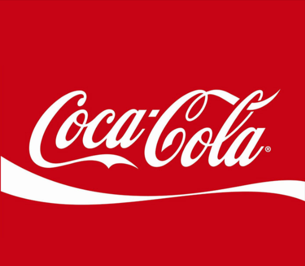
Use Matplotlib
# Display image.
plt.imshow(cb_img)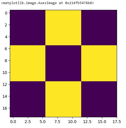
Even though the image was read in as a gray scale image, it won’t necessarily display in gray scale when using
imshow(). matplotlib uses different color maps and it’s possible that the gray scale color map is not set.
Force Grayscale
# Set color map to gray scale for proper rendering.
plt.imshow(cb_img, cmap="gray")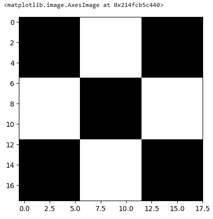
Fuzzy Image Below
- The image is shown below as well in OPenCV
# Display image.
plt.imshow(cb_img_fuzzy, cmap="gray")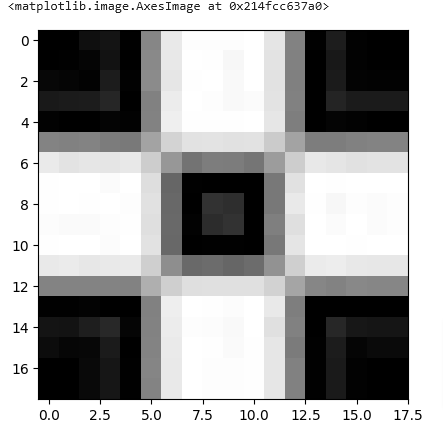
Display Colored Image
plt.imshow(coke_img)
#  What happened?
The color displayed above is different from the actual image. This is because matplotlib expects the image in RGB format whereas OpenCV stores images in BGR format. Thus, for correct display, we need to reverse the channels of the image. We will discuss about the channels in the sections below.
coke_img_channels_reversed = coke_img[:, :, ::-1]
plt.imshow(coke_img_channels_reversed)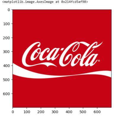
OpenCV
Read With OpenCV
OpenCV allows reading different types of images (JPG, PNG, etc). You can load grayscale images, color images or you can also load images with Alpha channel. It uses the cv2.imread() function which has the following syntax:
Syntax
retval = cv2.imread( filename[, flags] )retval: Is the image if it is successfully loaded. Otherwise it is None. This may happen if the filename is wrong or the file is corrupt.
The function has 1 required input argument and one optional flag:
filename: This can be an absolute or relative path. This is a mandatory argument.Flags: These flags are used to read an image in a particular format (for example, grayscale/color/with alpha channel). This is an optional argument with a default value ofcv2.IMREAD_COLORor1which loads the image as a color image.
Before we proceed with some examples, let’s also have a look at some of the flags available.
Flags
cv2.IMREAD_GRAYSCALEor0: Loads image in grayscale modecv2.IMREAD_COLORor1: Loads a color image. Any transparency of image will be neglected. It is the default flag.cv2.IMREAD_UNCHANGEDor-1: Loads image as such including alpha channel.
Documentation
Imread: Documentation linkImreadModes: Documentation link
Read as Grayscale
# Read image as gray scale.
cb_img = cv2.imread("checkerboard_18x18.png", 0)

# Print the image data (pixel values), element of a 2D numpy array.
# Each pixel value is 8-bits [0,255]
print(cb_img)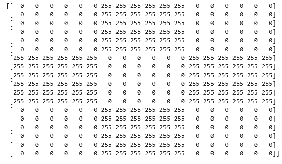
Image Attributes
# print the size  of image
print("Image size (H, W) is:", cb_img.shape)

# print data-type of image
print("Data type of image is:", cb_img.dtype)

# OUTPUT
Image size (H, W) is: (18, 18)
Data type of image is: uint8
Fuzzy Image
# Read image as gray scale.
cb_img_fuzzy = cv2.imread("checkerboard_fuzzy_18x18.jpg", 0)

# print image
print(cb_img_fuzzy)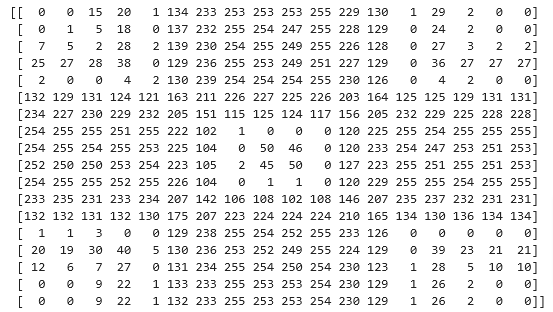
Color Image
- Let’s look at the attributes of the image viewed in ipython above
# Read in image
coke_img = cv2.imread("coca-cola-logo.png", 1)

# print the size  of image
print("Image size (H, W, C) is:", coke_img.shape)

# print data-type of image
print("Data type of image is:", coke_img.dtype)

# OUTPUT
Image size (H, W, C) is: (700, 700, 3)
Data type of image is: uint8
Splitting & Merging Colors
cv2.split()Divides a multi-channel array into several single-channel arrays.cv2.merge()Merges several arrays to make a single multi-channel array. All the input matrices must have the same size.
# Split the image into the B,G,R components
img_NZ_bgr = cv2.imread("New_Zealand_Lake.jpg", cv2.IMREAD_COLOR)
b, g, r = cv2.split(img_NZ_bgr)

# Show the channels
plt.figure(figsize=[20, 5])

plt.subplot(141);plt.imshow(r, cmap="gray");plt.title("Red Channel")
plt.subplot(142);plt.imshow(g, cmap="gray");plt.title("Green Channel")
plt.subplot(143);plt.imshow(b, cmap="gray");plt.title("Blue Channel")

# Merge the individual channels into a BGR image
imgMerged = cv2.merge((b, g, r))
# Show the merged output
plt.subplot(144)
plt.imshow(imgMerged[:, :, ::-1])
plt.title("Merged Output")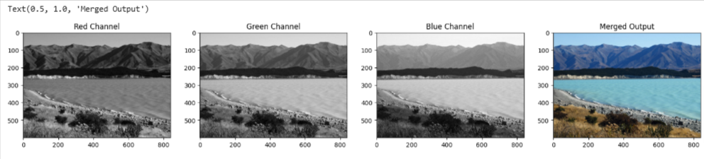
Converting Color
Converting to different Color Spaces
cv2.cvtColor() Converts an image from one color space to another. The function converts an input image from one color space to another. In case of a transformation to-from RGB color space, the order of the channels should be specified explicitly (RGB or BGR). Note that the default color format in OpenCV is often referred to as RGB but it is actually BGR (the bytes are reversed). So the first byte in a standard (24-bit) color image will be an 8-bit Blue component, the second byte will be Green, and the third byte will be Red. The fourth, fifth, and sixth bytes would then be the second pixel (Blue, then Green, then Red), and so on.
Function Syntax
dst = cv2.cvtColor( src, code )
dst: Is the output image of the same size and depth as src.
The function has 2 required arguments:
srcinput image: 8-bit unsigned, 16-bit unsigned ( CV_16UC… ), or single-precision floating-point.codecolor space conversion code (see ColorConversionCodes).
Changing from BGR to RGB
# OpenCV stores color channels in a differnet order than most other applications (BGR vs RGB).
img_NZ_rgb = cv2.cvtColor(img_NZ_bgr, cv2.COLOR_BGR2RGB)
plt.imshow(img_NZ_rgb)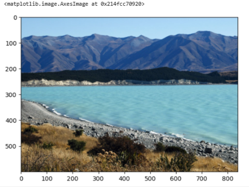
Changing to HSV Color
img_hsv = cv2.cvtColor(img_NZ_bgr, cv2.COLOR_BGR2HSV)

# Split the image into the H,S,V components
h,s,v = cv2.split(img_hsv)

# Show the channels
plt.figure(figsize=[20,5])
plt.subplot(141);plt.imshow(h, cmap="gray");plt.title("H Channel");
plt.subplot(142);plt.imshow(s, cmap="gray");plt.title("S Channel");
plt.subplot(143);plt.imshow(v, cmap="gray");plt.title("V Channel");
plt.subplot(144);plt.imshow(img_NZ_rgb);   plt.title("Original");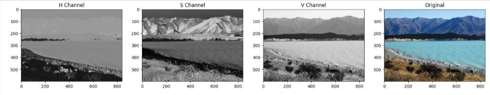
Modify Each Channel
h_new = h + 10
img_NZ_merged = cv2.merge((h_new, s, v))
img_NZ_rgb = cv2.cvtColor(img_NZ_merged, cv2.COLOR_HSV2RGB)

# Show the channels
plt.figure(figsize=[20,5])
plt.subplot(141);plt.imshow(h, cmap="gray");plt.title("H Channel");
plt.subplot(142);plt.imshow(s, cmap="gray");plt.title("S Channel");
plt.subplot(143);plt.imshow(v, cmap="gray");plt.title("V Channel");
plt.subplot(144);plt.imshow(img_NZ_rgb);   plt.title("Original");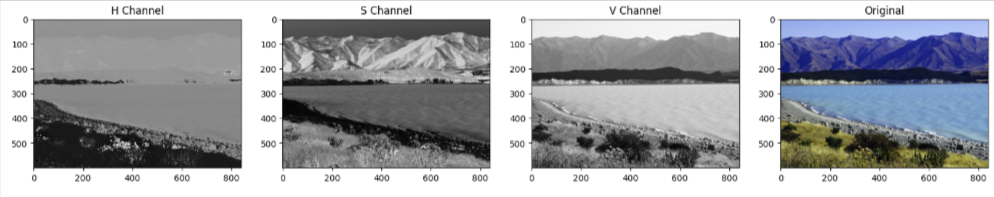
Saving Images
Saving the image is as trivial as reading an image in OpenCV. We use the function cv2.imwrite() with two arguments. The first one is the filename, second argument is the image object.
The function imwrite saves the image to the specified file. The image format is chosen based on the filename extension (see cv::imread for the list of extensions). In general, only 8-bit single-channel or 3-channel (with ‘BGR’ channel order) images can be saved using this function (see the OpenCV documentation for further details).
Syntax
cv2.imwrite( filename, img[, params] )The function has 2 required arguments:
filename: This can be an absolute or relative path.img: Image or Images to be saved.
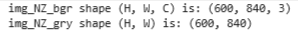
# save the image
cv2.imwrite("New_Zealand_Lake_SAVED.png", img_NZ_bgr)

Image(filename='New_Zealand_Lake_SAVED.png')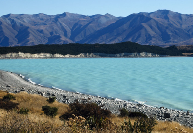
# read the image as Color
img_NZ_bgr = cv2.imread("New_Zealand_Lake_SAVED.png", cv2.IMREAD_COLOR)
print("img_NZ_bgr shape (H, W, C) is:", img_NZ_bgr.shape)

# read the image as Grayscaled
img_NZ_gry = cv2.imread("New_Zealand_Lake_SAVED.png", cv2.IMREAD_GRAYSCALE)
print("img_NZ_gry shape (H, W) is:", img_NZ_gry.shape)