~AI\computer_vision\od_projects\opencv_learn>venv_opencv\Scripts\activate

(venv_opencv) ~AI\computer_vision\od_projects\opencv_learn>jupyter notebookImage Annotation
In this page we will cover how to annotate images using OpenCV. We will learn how to peform the following annotations to images.
- Draw lines
- Draw circles
- Draw rectangles
- Add text
These are useful when you want to annotate your results for presentations or show a demo of your application. Annotations can also be useful during development and debugging.
Setup
Reminder:
- Since I am trying to keep all notebooks organized I will go into my directory
- Activate the appropriate venv_opencv
- From an activated venv I will open jupyter notebook (see the code below)
- Create a new notebook: image_manipulation_opencv
- Choose “Py venv_opencv” kernel
.
Import Libraries
import os
import cv2
import matplotlib
import numpy as np
import matplotlib.pyplot as plt

from zipfile import ZipFile
from urllib.request import urlretrieve

matplotlib.rcParams['figure.figsize'] = (9.0, 9.0)

%matplotlib inline
Import Assets
def download_and_unzip(url, save_path):
    print(f"Downloading and extracting assests....", end="")

    # Downloading zip file using urllib package.
    urlretrieve(url, save_path)

    try:
        # Extracting zip file using the zipfile package.
        with ZipFile(save_path) as z:
            # Extract ZIP file contents in the same directory.
            z.extractall(os.path.split(save_path)[0])

        print("Done")

    except Exception as e:
        print("\nInvalid file.", e)
# provide url and call function
URL = r"https://www.dropbox.com/s/48hboi1m4crv1tl/opencv_bootcamp_assets_NB3.zip?dl=1"
asset_zip_path = os.path.join(os.getcwd(), "opencv_bootcamp_assets_NB3.zip")
# Download if assest ZIP does not exists.
if not os.path.exists(asset_zip_path):
download_and_unzip(URL, asset_zip_path) Draw Line
Read Image
# Read in an image
image = cv2.imread("Apollo_11_Launch.jpg", cv2.IMREAD_COLOR)

# Display the original image
plt.imshow(image[:, :, ::-1])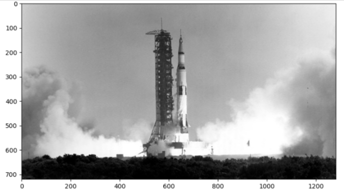
Syntax
img = cv2.line(img, pt1, pt2, color[, thickness[, lineType[, shift]]])img: The output image that has been annotated.
The function has 4 required arguments:
img: Image on which we will draw a linept1: First point(x,y location) of the line segmentpt2: Second point of the line segmentcolor: Color of the line which will be drawn
Other optional arguments that are important for us to know include:
thickness: Integer specifying the line thickness. Default value is 1.lineType: Type of the line. Default value is 8 which stands for an 8-connected line. Usually, cv2.LINE_AA (antialiased or smooth line) is used for the lineType.- Documentation
imageLine = image.copy()

# The line starts from (200,100) and ends at (400,100)
# The color of the line is YELLOW (Recall that OpenCV uses BGR format)
# Thickness of line is 5px
# Linetype is cv2.LINE_AA

cv2.line(imageLine, (200, 100), (400, 100), (0, 255, 255), thickness=5, lineType=cv2.LINE_AA);

# Display the image
plt.imshow(imageLine[:,:,::-1])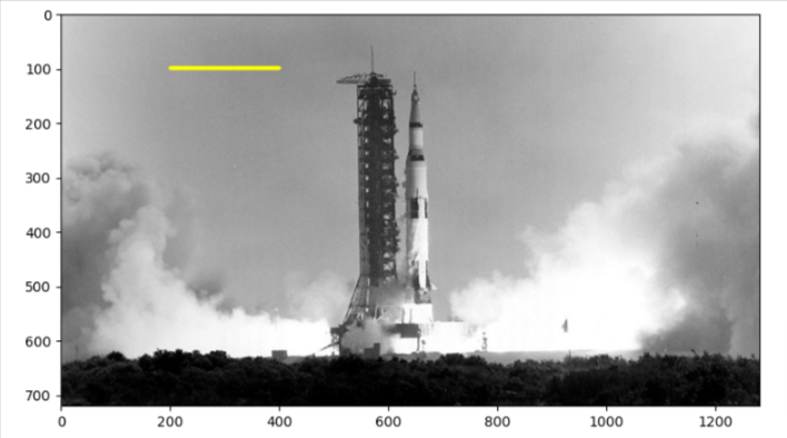
Draw Circle
Syntax
img = cv2.circle(img, center, radius, color[, thickness[, lineType[, shift]]])img: The output image that has been annotated.
The function has 4 required arguments:
img: Image on which we will draw a linecenter: Center of the circleradius: Radius of the circlecolor: Color of the circle which will be drawn
Next, let’s check out the (optional) arguments which we are going to use quite extensively.
thickness: Thickness of the circle outline (if positive). If a negative value is supplied for this argument, it will result in a filled circle.lineType: Type of the circle boundary. This is exact same as lineType argument in cv2.line
# Draw a circle
imageCircle = image.copy()

cv2.circle(imageCircle, (900,500), 100, (0, 0, 255), thickness=5, lineType=cv2.LINE_AA);

# Display the image
plt.imshow(imageCircle[:,:,::-1])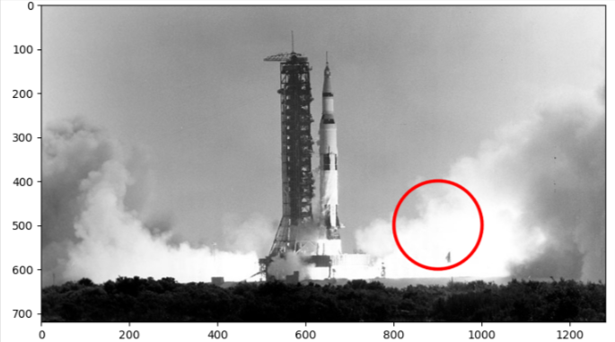
Draw Rectangle
Syntax
img = cv2.rectangle(img, pt1, pt2, color[, thickness[, lineType[, shift]]])img: The output image that has been annotated.
The function has 4 required arguments:
img: Image on which the rectangle is to be drawn.pt1: Vertex of the rectangle. Usually we use the top-left vertex here.pt2: Vertex of the rectangle opposite to pt1. Usually we use the bottom-right vertex here.color: Rectangle color
Next, let’s check out the (optional) arguments which we are going to use quite extensively.
thickness: Thickness of the rectangle outline (if positive). If a negative value is supplied for this argument, it will result in a filled rectangle.lineType: Type of the rectangle boundary. This is exact same as lineType argument in cv2.line
# Draw a rectangle (thickness is a positive integer)
imageRectangle = image.copy()
# we'll have the upper corner at 500,100 and lower right corner at 700,600 with color purple...
cv2.rectangle(imageRectangle, (500, 100), (700, 600), (255, 0, 255), thickness=5, lineType=cv2.LINE_8)

# Display the image
plt.imshow(imageRectangle)

# can use to reverse it
#plt.imshow(imageRectangle[:, :, ::-1])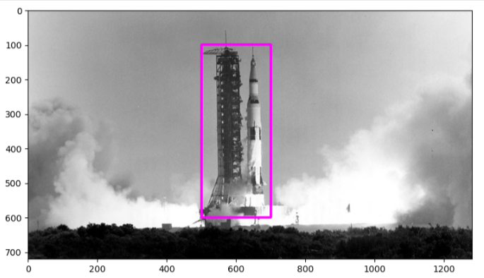
Add Text
Syntax
img = cv2.putText(img, text, org, fontFace, fontScale, color[, thickness[, lineType[, bottomLeftOrigin]]])img: The output image that has been annotated.
The function has 6 required arguments:
img: Image on which the text has to be written.text: Text string to be written.org: Bottom-left corner of the text string on where to place in the image.fontFace: Font typefontScale: Font scale factor that is multiplied by the font-specific base size.color: Font color
Other optional arguments that are important for us to know include:
thickness: Integer specifying the line thickness for the text. Default value is 1.lineType: Type of the line. Default value is 8 which stands for an 8-connected line. Usually, cv2.LINE_AA (antialiased or smooth line) is used for the lineType.
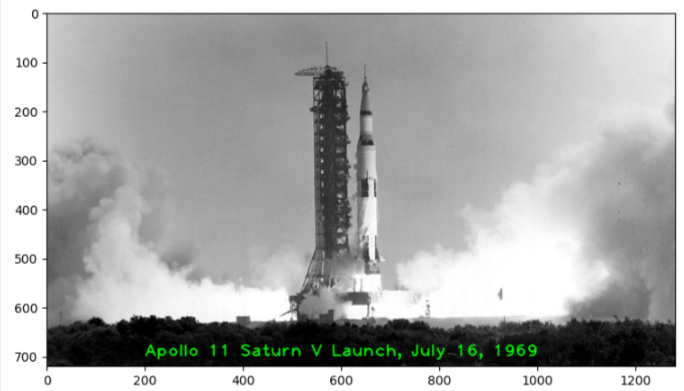
imageText = image.copy()
text = "Apollo 11 Saturn V Launch, July 16, 1969"
fontScale = 2.3
fontFace = cv2.FONT_HERSHEY_PLAIN
fontColor = (0, 255, 0)
fontThickness = 2

cv2.putText(imageText, text, (200, 700), fontFace, fontScale, fontColor, fontThickness, cv2.LINE_AA);

# Display the image
plt.imshow(imageText[:, :, ::-1])